Efficiency#
We know that some programs run faster than others. However, the speed the program runs at depends on many things, including the computer it is running on, the other programs that may be running at the same time, and the supporting software (e.g., the particular version of Python and the underlying operating system), as well as the input data provided to the program.
We might be able to measure the performance of a particular execution of the program on a particular system and determine that it took 3.5 seconds. Sometimes we do need that kind of measurement, but we also need a more general way to talk about the efficiency of the program that will tell us something about its relative speed on other data sets and other computers. That is what we call algorithmic efficiency.
It’s the curve that counts#
Instead of counting seconds required to execute a program on a particular data set on a particular computer, we characterize algorithmic efficiency by a relation between problem size and execution time. For example, if the time t required to execute a program could be described by an equation \(t = mx + b\), where m is a constant, x is a measure of the problem size and b is a constant (e.g., it might be some fixed start-up time that does not depend on the input data), we would say that the program’s performance is linear in x, because \(t = mx + b\) is the equation of a straight line.
We generally care most about how fast or slow a program is when given a very large problem to work on. For very large programs, constant factors like m and b matter less than the exponent of the leading term. For example, if we have one program whose performance is described by \(t_1 = mx + b\), and another program whose performance is described by \(t_2 = nx^2 + c\), we typically prefer the former even if \(m \gg n\) and \(b \gg c\). \(t_1\) may be larger when \(x\) is small, but for very large values of \(x\), \(t_2\) will certainly be larger.
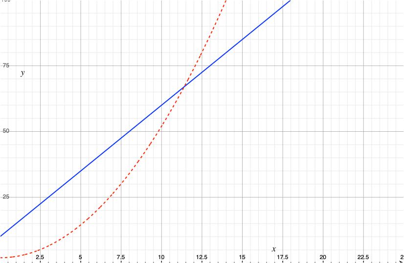
Fig. 5 A program that requires \(0.5x^2 + 2\) operations for a problem of size \(x\) (dotted line) may be faster that a program that requires \(5x + 10\) operations (solid line) when \(x\) is small, but the lines cross around \(x = 12\) and thereafter the quadratic function grows much faster.#
We seldom care whether our program takes a hundredth of a second or a tenth of a second on a small problem. Our focus is on efficiency with large problem sizes, where performance is more likely to be an issue. For example, consider the following function for determining whether a list of integers contains any duplicate items:
def has_dups(l: list[int]) -> bool:
  """Is l[i] == l[j] for i != j?"""
  for i in range(len(l)):
    # Only need to compare items after position i
    for j in range(i+1,len(l)):
      if l[i] == l[j]:
        return True
  return False

print(f"Expecting True: {has_dups([0, 7, 3, 5, 9, 8, 17, 3, 2])}")
print(f"Expecting False: {has_dups([0, 7, 3, 5, 9, 8, 17, 13, 2])}")
Expecting True: True
Expecting False: False
The function seems simple and clear, and it works well enough for
short lists like the test cases. But how long could has_dups take
on a much longer list, say 10,001 items? If there are no duplicate
elements, the outer loop will run 10,001 times, which is not bad by
itself. On the first iteration of the outer loop, the inner loop
will execute 10,000 times. On the second, it will execute 9,999 times,
then 9,998 times for the second time through the outer loop, and so
on. The total number of times the the comparison l[i] == l[j]
will be executed is \(1 + 2 + 3 + \ldots + 10,000\), which is
\(10,000 (10,000 + 1) /2\), or approximately 50,000,000. For a list
of \(n\) items, the total execution time is proportional to \(n^2\); we
say it is quadratic in list size.
If we graphed the time required by this first version of has_dups
on the y axis, with list length as the x axis, we would see the
shape of a parabola.
We can make a version of has_dups that works much more
efficiently on long lists.
def has_dups(l: list[int]) -> bool:
  """Is l[i] == l[j] for i != j?
  This version is much faster for long lists.
  """
  m = sorted(l)
  # Any duplicate items are now adjacent
  for i in range(len(m) - 1):
    if m[i] == m[i + 1]:
      return True
  return False

print(f"Expecting True: {has_dups([0, 7, 3, 5, 9, 8, 17, 3, 2])}")
print(f"Expecting False: {has_dups([0, 7, 3, 5, 9, 8, 17, 13, 2])}")
Expecting True: True
Expecting False: False
The built-in Python function sorted
requires time proportional to \(n \log_2 n\) to sort a list with \(n\)
elements. For 10,000 elements, this is approximately
\(10,000 \times 13 \times k\), where \(k\) is a constant and independent
of list length. If we graphed the time required by this second
version of has_dups, we would see a line that curves slightly
upward, but far less steeply than the parabola describing the first
version.
If \(k\) is fairly large (which depends on details of
how sorted is implemented in Python), it is possible that our
first implementation of has_dups could be faster for very short
lists like those in our test cases … but who cares when both are
so fast? Our second implementation will be far faster for a list
with 10,000 elements. If we try has_dups on a list with a million
elements, the second version will be execute reasonably quickly,
while the first will be impractical. We therefore prefer the second
version.
Algorithmic efficiency classes#
If we ignore coefficients and constants and focus just on the shapes of the curves we see if we graph execution time against problem size, most of our programs and functions will fall into one of several efficiency classes. From fastest to slowest (on large problems), these are:
Constant time: The execution time of the program does not depend on the size of the problem. We seldom write whole programs that execute in constant time, but a program might include some functions whose execution time is independent of problem size.
For example, the built-inlenfunction n Python does not depend on the length of the list.Logarithmic time: The execution time of the function is proportional to the logarithm of the problem size. We can seldom achieve logarithmic time for a whole program, since we must at least read the data it processes (already that requires linear time), but sometimes an individual function can have logarithmic performance. Binary search is an example of an algorithm that requires logarithmic time.
Linear time: The execution time of the program or function is directly proportional to problem size. For example, the built-in function
maxhas performance that is linear in the length of the list it is given.Log-linear time: Execution time proportional to the problem size times the logarithm of problem size. For example, the built-in Python function
sortedhas log-linear performance.Quadratic time: Performance is proportional to the square of the problem size. A quadratic time algorithm may be perfectly fine if we know the problem size can never be large, but it is apt to be unsatisfactory for very large data sets.
Cubic, quartic, … polynomial time: Some functions could require time proportional to \(n^3\), \(n^4\), etc., a polynomial with a leading exponent larger than 2. There are some problems for which this is the best we can do, but these algorithms are unlikely to be satisfactory for large problems.
Exponential: If the performance of a function or program is proportional to a function with problem size in the exponent, e.g., \(2^n\), we say it is exponential. Consider for example an algorithm that must check every subset of a set of \(n\) elements. There are \(2^n\) such subsets.
Functions that require time that is exponential in problem size can be applied only to very small problems, as even \(2^{20}\) is over a million, and \(2^{32}\) is over 4 billion.
Note that for a programmer, “exponential” is not just a synonym for “very big”. It has a precise meaning. Computer scientists use the term hard problem to mean a problem for which the only possible solutions require exponential time. We may cringe when others use the term “exponential” to mean “really big”, but we are ok with others using the term “hard” in more informal senses.
Fast and slow patterns#
A constant time algorithm can usually be written without any loops, or with a loop that does not depend on the input data.
A linear time algorithm usually involves a loop that depends on problem size, e.g., a loop through the elements of a list. Each step within the loop must execute in constant time.
A loop that requires linear time, followed by another loop that requires linear time, is still linear time.
When we put one loop inside another loop (nested), the complexity
of the combination is the product of the complexities of the
individual loops. Our first attempt at has_dups nested loops that
were each linear in the length of a list, resulting in quadratic
complexity.
Nested loops are not always as obvious as our first has_dups. We
might write a function with a single loop through the elements of a
list, and in the body of that loop we might call another function
that also loops through the list. We do not see syntactic
nesting of one loop inside another, but they are semantically nested.
Perspective#
Most of the code we write is not performance-critical. Often we can write simple, readable code that is good enough without thinking much about it. Typically we try to write code that is straightforward, understandable, and not horrible with respect to efficiency.
But we must be more careful. Accidentally writing a function whose execution time is quadratic in the size of the data it processes can be a logic bomb waiting to go off at an inconvenient time. Such a function may appear fine in testing, because test cases are typically small. It may even be acceptable most of the time in production use, but then one day when it encounters a larger problem and slows an application unacceptably, it will likely be while the system is under heavy load.
Algorithmic efficiency is one key consideration for performance-critical systems, but not the only consideration. Algorithm design focusing on the shape of the curve is typically followed by performance tuning to squeeze out additional constant factors. Halving the time required by some function is “only” a constant factor, but halving the time required for a large scientific simulation or halving the hosting expenses of a large internet-based business is significant.
If you continue with computer science courses, you will dig much deeper into devising and analyzing efficient functions in data structures and algorithms courses. Our treatment so far is informal, but you should be able to do some basic reasoning and distinguish between constant time, linear time, and quadratic algorithms on lists.
Binary search#
We looked at differences between linear time algorithms for lists and quadratic time algorithms, which typically involve nested loops. Can we get even more efficient than linear time? The next section describes binary search, a way of achieving logarithmic complexity provided a list is in sorted order.